AMPL Shell- Example of Use

Two products can be produced at a steel mill: bands and coils

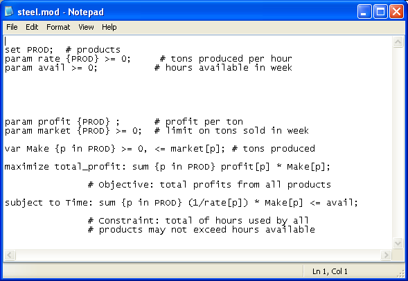
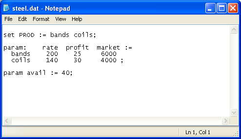
We can make 200 tons of bands in an hour; the profit for each ton is 25 dollars; the demand is 6000 tons. We must make at least 1000 tons of this product.

We can make 140 tons of coils in an hour; the profit for each ton is 30 dollars; the demand is 4000 tons. We must make at least 2000 tons of this product.

We have 40 hours of production time available.

The goal is to design a production plan to maximize total profit.

If you have added the AMPL installation directory to the search path, you can run AMPL from any directory. Otherwise, run AMPL by moving to the AMPL directory and typing ampl at the shell prompt.

At the ampl: prompt, you can type any AMPL language statement, or any of the commands described in Section A.13 of the book AMPL: A Modeling Language for Mathematical Programming. To end the session, type quit; at the ampl: prompt.

Generally, you will edit your model and data (both expressed using AMPL language statements) in a text editor, and type commands at the ampl: prompt to load your model and data, solve a problem, and inspect the results. Although you could type in the statements of a model at the ampl: prompt, AMPL does not include a built-in text editor, so you cannot use AMPL commands to edit the statements you have previously entered. Microsoft Windows users (on PCs) and XWindows users (on Unix systems) should open separate windows for editing files and running AMPL.

If you cannot open multiple windows on your desktop, you can use AMPL’s shell command to invoke an editor from within AMPL. You can use any editor that saves files in ASCII format. Windows command-line (DOS) users can use edit or notepad and Unix users vi or emacs. If you are using edit under DOS, for instance, you can type:

ampl: shell ‘edit steel.dat’;

You can use any text editors to edit your model and data files. Use editor menus and commands to edit your file, then save it and exit the editor.

At the ampl: prompt you can type new AMPL commands, such as:

ampl: reset data;
ampl: data steel.dat;

Note that editing a file in a text editor does not affect your AMPL session until you explicitly reload the edited file, as shown above.

If you have previously developed a model and its data, and would like to solve it and display the results automatically, you can create a file containing the commands you would like AMPL to execute, and specify that file at the command line when you run AMPL. For example, you might create a file called steel.run, containing the commands:

model steel.mod;
data steel.dat;
option solver cplexamp;
solve;
display Make >steel.ans;
Note that this assumes that steel.run is in the same directory as the model and data files, and that AMPL can be found on the path.

You can then run AMPL as follows:

C:\> ampl steel.run

A more flexible approach, which is a commonly followed convention among AMPL users, is to put just the AMPL commands (the last three lines in the example above) in a file with the *.run extension. You can then type:

C:\> ampl steel.mod steel.dat steel.run

which accomplishes the same thing as:

C:\> ampl
ampl: include steel.mod;
ampl: include steel.dat;
ampl: include steel.run;
ampl: quit;
C:\>

If you intend to load several files and solve a problem, but you want to type a few interactive commands in the middle of the process, type the character – in place of a filename. AMPL processes the files on the command line from left to right; when it encounters the – symbol it displays the ampl: prompt and accepts commands until you type end;. For example, you could type:

C:\> ampl steel.mod steel.dat – steel.run
ampl: let avail := 50;
ampl: end;

This will solve the problem as before, but with the parameter avail set to 50 instead of 40 (the value specified in steel.dat). To start AMPL, load a model and data file, and wait for your interactive commands, type:

AMPL’s solver interface supports linear, nonlinear, and mixed integer models with no built-in size limitations. This interface is rich enough to support many of the features used by advanced solvers to improve performance and solution accuracy, such as piecewise-linear constructs, representation of network problems, and automatic differentiation of nonlinear functions. To take advantage of these features, solvers must be written to utilize AMPL’s interface.

You choose a solver for a particular problem by giving its executable filename in the AMPL option solver command. For example, to use the (AMPL-compatible) CPLEX solver, type:

ampl: option solver cplexamp;

Most solvers have algorithmic options, such as CPLEX with its Mixed Integer and Barrier options. In these cases, you give the solver executable name to AMPL (for example, with option solver cplexamp); the solver will determine, from the problem characteristics as passed by AMPL (for example, a quadratic objective or integer variables) as well as solver options you specify, which algorithmic options will be used.

You can specify option settings for a particular solver through the AMPL option command. (CPLEX-specific directives are described later in this document.) Since all solvers provide default settings for their options, this is necessary only when your problem requires certain nondefault settings in order to solve, or when certain settings yield improved performance or solution accuracy.

To specify solver options, enter

option solver_options ‘settings’;

Where solver is replaced by the name of the solver you are using. This approach allows you to set up different options for each solver you use and to switch among them by simply choosing the appropriate solver with the option solver command. For example:

ampl: option cplex_options ‘relax scale=1’;

Solver options consist of an identifier alone, or an identifier followed by an = sign and a value. Some solvers treat uppercase and lowercase versions of an option identifier as equivalent, while others are sensitive to case, so that RELAX is not the same as relax, for example.

Solver option settings can easily become long enough to stretch over more than one line. In such cases you can either continue a single quoted string by placing a \ character at the end of each line, as in:

ampl: option cplex_options ‘crash=0 dual \
ampl? feasibility=1.0e-8 scale=1 \
ampl? lpiterlim=100’;

Or you can write a series of individually quoted strings, which will be concatenated automatically by AMPL, as in:

ampl: option cplex_options ‘crash=0 dual’
ampl? ‘ feasibility=1.0e-8 scale=1’
ampl? ‘ lpiterlim=100’;

If you use the latter approach, be sure to include spaces at the beginning or end of the individual strings, so that the identifiers will be separated by spaces when all of the strings are concatenated.

Often you will want to add solver options to the set you are currently using. If you simply type a command such as option solver_options ‘new options’; however, you will overwrite the existing option settings. To avoid this problem, you can use AMPL’s $ notation for options: the symbol $option_name is replaced by the current value of option_name. To add an optimality tolerance to the CPLEX options in the above example, you would write:

ampl: option cplex_options $cplex_options
ampl? ‘ optimality=1.0e-8’;

When you type solve; AMPL processes your model and data to create a temporary problem file, such as steel.nl, which will be read by the solver. It then loads and executes the solver program, which is responsible for creating a solution file such as steel.sol. AMPL reads the solution file and makes the solution values available through the variable, constraint, and objective names you have declared in your AMPL model. Unless you specify otherwise, AMPL then deletes the temporary problem and solution files.

You can display the solution information, for example the values of the decision variables and constraints, in your AMPL session with commands such as display. For example, if you have just solved a problem created from steel.mod and steel.dat, you could type:

ampl: display Make, Time;

To save this output in a file, you can use redirection:

ampl: display Make, Time > mysol.txt;

Note that when you simply mention the name of a constraint in a display statement, AMPL will display the dual value (shadow price) of that constraint, not its left-hand side value. You can use the AMPL suffix notation to display the left-hand side value, as described in the book AMPL: A Modeling Language for Mathematical Programming.